Machine learning analysis of cardiovascular risk factors and their associations with hearing loss

Study design and data source

We conducted a retrospective analysis of data from the NHANES from 2012–2018. NHANES is an ongoing cross-sectional survey conducted by the National Center for Health Statistics to assess the health and nutritional status of adults and children in the US. The survey combines interviews, physical examinations, and laboratory tests using a complex, multistage probability sampling design to obtain nationally representative samples. The audiometry component measures hearing thresholds for speech and pure tone frequencies, allowing assessment of hearing function. NHANES data are publicly available at https://www.cdc.gov/nchs/nhanes/about_nhanes.htm.

From 28,874 NHANES participants, 20,988 were excluded due to age < 20 years, incomplete audiometric data, or self-reported hearing loss/related conditions. Exclusions covered hereditary or genetic factors, certain infections, specific medical conditions, medications, and noise exposure, including conditions such as congenital hearing loss, auditory neuropathy spectrum disorder, Meniere’s disease, otosclerosis, and noise-induced hearing loss. The final sample comprised 7,996 participants ≥ 20 years with complete audiometric data and no self-reported hearing loss conditions. By excluding individuals with self-reported hearing loss conditions, we aimed to focus the analysis on predicting the onset of hearing impairment, rather than examining factors associated with pre-existing diagnosed hearing loss. Individuals with self-reported hearing loss may have different etiologies and risk factor profiles, which could introduce confounding factors and bias the predictive models. This sample was obtained by first removing those with missing audiometric data (17,849 excluded), then excluding those < 20 years (3,029 excluded), and after that excluding self-reported hearing loss/related conditions (110 excluded) (Fig. 1).

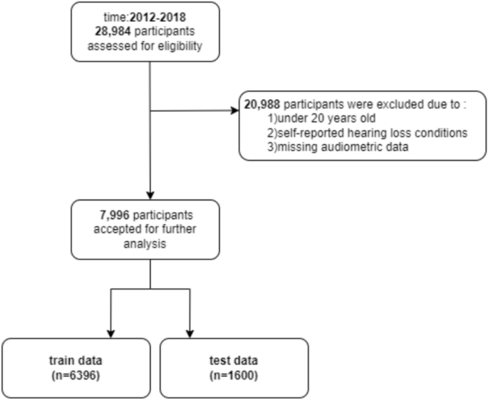
Flow diagram of the cohort study.

To develop our predictive model for hearing impairment, we conducted an extensive literature review to identify key demographic, clinical, behavioural, and environmental risk factors associated with CVD that may impact hearing health. The CVD risk factors, CVD health metrics, and CVDs were selected based on the guidelines developed by the American College of Cardiology (ACC), the American Heart Association (AHA), and the Framingham Heart Study^22,23. Based on this comprehensive review, we selected 50 relevant variables consistently measured in the NHANES 2012–2018 dataset, allowing assessment of main hearing loss risk factors as well as CVD risk factors in a robust, nationally representative population sample (Table S1).

The demographic attributes included age, gender, race/ethnicity, poverty income ratio and education level. CVD risk factors and history captured self-reported diagnoses of conditions like diabetes, prediabetes, hyperlipidemia, and hypertension as well as related prescription medication use. Clinical biomarkers measured included glycosylated hemoglobin (HbA1c), fasting plasma glucose, serum lipids (HDL, LDL, total cholesterol), blood pressure, anthropometric data (body mass index, waist circumference), and cotinine levels. Dietary intake variables from 24-h recalls focused on components relevant to the Dietary Approaches to Stop Hypertension (DASH) diet. Physical activity domains included transportation, leisure activities, and exercise duration/intensity. Questions on smoking and alcohol consumption assessed lifetime use and current intake. Access to healthcare was represented by insurance status and provider counseling on conditions like hyperlipidemia and hypertension. Cardiovascular-associated factor data were obtained from the closest available clinical encounter in the NHANES dataset, which may not correspond to the exact day of the audiological evaluation, potentially introducing variability due to day-to-day fluctuations in these measures.

Primary outcome

We defined hearing impairment based on the pure-tone average (PTA) audiometry, calculated as the mean hearing threshold in decibels hearing level (dB HL) at 500, 1000, 2000, and 4000 Hz for better ear on NHANES audiometry testing. Aligning with American Speech-Language-Hearing Association (ASHA) guidelines, we categorized hearing thresholds into three distinct groups for analysis:

Normal vs. Abnormal Hearing: Threshold set at > 16 dB HL to identify deviations from normal hearing.

Slight vs. More than Slight Impairment: Threshold set at > 25 dB HL to distinguish slight/normal impairment from more significant impairment.

Severe vs. Less than Severe Impairment: Threshold set at > 40 dB HL to identify severe hearing loss^2,24. Our primary analysis focused on the > 25 dB HL threshold to classify binary hearing impairment. Additionally, supplementary analyses applied the > 16 dB HL and > 40 dB HL thresholds to explore slight impairment and severe hearing loss, respectively.

Additionally, we developed ML regression models to predict patients’ precise PTA audiometry values, mapped onto the above clinical categories. By modelling PTA as a continuous measure, we aimed to quantify impairment severity across the full range observed in the NHANES cohort (Fig. 2).

Proposed methodology. Overview of the preprocessing and modeling methodology. Data preprocessing involved applying tailored transformations to each column using a column transformer, which allows numerical data to be normalized and categorical data to be encoded. The fit-transform process learns the required parameters from the training data and applies them to both training and test datasets, ensuring consistency in preprocessing. These steps prepared the data for downstream machine learning models, including custom-designed classifiers and regressors tailored for hearing loss prediction.

Data preprocessing

The NHANES dataset underwent preprocessing for predictive modelling. Binary features were converted to 0/1, while rejected and unknown responses were marked as missing. The dataset of 7,996 patients was split 80/20 for training and testing. Variables and patients with over 20% missing data were excluded. For the remaining missing values, we first assessed the missingness mechanism by adding missing indicators and evaluating Spearman’s correlation between missing indicators and observed values. The analysis revealed no significant correlation, indicating that missing values were completely at random (MCAR) (Figure S1). Based on the findings of missing analysis, missing categorical variables were imputed using mode, and missing numerical variables were imputed using mean to preserve dataset integrity while preparing it for analysis^25,26,27,28. The method of stratified random sampling used in this study ensured a balanced division of the 7,996 participants into training and test cohorts. By creating strata based on key variables such as age, gender, and race/ethnicity, and then performing random sampling within each stratum, the approach maintained the proportional representation of these demographic features across both cohorts. To validate the comparability, chi-square tests confirmed uniform distributions for categorical variables, while continuous variables underwent Kolmogorov–Smirnov and Mann–Whitney U tests to ensure consistency in distributional shapes between the two sets. This method reduced bias and enhanced the generalizability of the predictive models developed.

Subsequent transformations included the one-hot encoding of categorical and ordinal features to convert them into a machine-readable numerical format. Numerical variables were subjected to scalar normalization to mitigate the impact of outliers, ensuring a balanced and equitable dataset for model training²⁹. To address the class imbalance, present in the dataset, where the number of individuals without hearing impairment significantly outnumbered those with hearing impairment, we employed the Synthetic Minority Over-sampling Technique (SMOTE). SMOTE is a well-established oversampling approach that generates synthetic instances of the minority class by interpolating between existing minority instances and their nearest neighbors³⁰. This technique has been proven effective in improving the performance of classification models on imbalanced datasets by preventing the majority class from dominating the learning process. The SMOTE algorithm was applied separately to the training set to generate synthetic minority class samples for each of the three hearing impairment thresholds (> 25 dB HL, > 16 dB HL, > 40 dB HL). This oversampling approach ensured that the training sets used for model development were balanced, with equal representation of the positive and negative classes for each hearing impairment classification task. The number of synthetic minority class samples generated by SMOTE was determined through a grid search, optimizing for the target class distribution that yielded the best overall model performance metrics on the held-out test set.

In this study, we employed Lasso regression as a means of feature selection to enhance the predictive performance of our model and to identify the most significant predictors of hearing impairment. Lasso, known for its capacity to reduce model complexity by penalizing the absolute size of regression coefficients, can effectively zero out less relevant features, thereby facilitating a more interpretable and streamlined model. We chose Lasso given its proven efficacy in handling datasets with potential multicollinearity and ability to perform feature selection from numerous predictors. We tuned the Lasso model by setting the hyperparameter, alpha, to 0.95. This specific value was chosen to balance model complexity and predictive accuracy, ensuring that only features with substantial contribution to the prediction of hearing impairment were retained³¹.

ML algorithms

To predict both the continuous PTA values and categorical hearing impairment thresholds, we evaluated an array of supervised ML algorithms. For regression modelling of the precise PTA outcome, we benchmarked linear models (Linear Regression), tree-based ensembles (Random Forest, Gradient Boosting, XGBoost, LightGBM), and multi-layer feedforward neural networks (MLP). Additionally, we employed a Multi-Layer Neural Network (MLNN), the architecture of which is detailed in a subsequent section. Classifiers explored for the dichotomous impairment assessment included logistic regression alongside the ensemble methods Random Forest, XGBoost, Gradient Boosting, CatBoost, and LightGBM^32,33,34.

Our models were constructed using Python (version 3.9.12; Python Software Foundation) and a collection of Python libraries, specifically numpy, pandas, matplotlib, sklearn, imblearn, xgboost, Keras, lightgbm, and catboost. The ensemble of models comprised RandomForestClassifier, RandomForestRegressor, XGBoost’s XGBClassifier, XGBRegressor, GradientBoostingClassifier, GradientBoostingRegressor, LogisticRegression, LinearRegression, MLPClassifier, MLPRegressor, LightGBM’s LGBMClassifier, LGBMRegressor, shap, and CatBoostClassifier (Table 1)^35,36.

MLNN architecture

We developed a multi-layer feedforward neural network for predicting PTA audiometry using the Keras API with TensorFlow 2.0 backend. The network comprised an input layer, an output layer, and four dense layers containing 32, 32, 16, and 16 nodes respectively. Rectified linear unit (ReLU) activation was applied on the hidden layers, while the output layer had a linear activation function for regressing the continuous PTA value. This choice was determined as part of the hyperparameter optimization process, as detailed in Table S2.

Dropout layers with a rate of 0.2 were used after the first and third dense layers to introduce regularization and improve generalization performance. We compiled the model using mean absolute error (MAE) loss, Adaptive Moment Estimation (Adam) optimization, and a batch size of 32.

This configuration was trained for 100 epochs while tracking performance on a held-out validation split. Using early stopping, training concluded early at 15 epochs upon observing a plateau in validation loss improvement. The final MLNN comprised 8,100 tunable parameters, achieving optimal generalizability to unseen data. Our multi-layer feedforward network for predicting continuous PTA values is outlined in Fig. 3. It depicts the propagation of input data x through four dense hidden layers, applying rectified linear activations and dropout regulation, before culminating in a linear output layer to regress the PTA outcome ŷ.

Evaluation of model performance

We evaluated model performance using several metrics tailored to the regression and classification tasks, accounting for the imbalanced nature of our dataset.

For the regression models predicting continuous PTA, we focused on mean absolute error (MAE), and root mean squared error (RMSE). These metrics provided a robust framework for quantifying the deviation of our model predictions from the actual values, thus offering a clear picture of model accuracy and the consistency of its predictions. RMSE is particularly useful in highlighting the impact of outliers on model performance, while MAE offers a straightforward, interpretable measure of average error magnitude across predictions. Lower values indicate better model fit and prediction accuracy.

The classification models used the speech-frequency pure-tone average (PTA) thresholds as the ground truth for determining hearing impairment categories. These thresholds (> 25 dB HL, > 16 dB HL, and > 40 dB HL), previously defined in the Primary Outcome subsection, were applied to categorize participants into distinct hearing impairment groups for the classification tasks. For our classification models based on PTA thresholds, accuracy alone was an insufficient metric given the class imbalance. In addition to accuracy, we considered the F1-score, the area under the receiver operating characteristic curve (AUCROC), and the area under the precision-recall curve (AUPRC). AUCROC and AUPRC provided valuable insights into the models’ ability to discriminate between classes, with AUPRC being particularly useful for evaluating the performance of the minority class³⁷. We also examined specificity, which measured the proportion of true negatives correctly identified, and sensitivity, which quantified the true positive rate. The F1-score balanced precision and recall, emphasizing minimizing both false positives and false negatives – an important consideration for this clinical prediction task³⁸.

We utilized stratified fivefold cross-validation repeated across 5 iterations on the NHANES training set to derive stable estimates of the above metrics (Fig. 2), including 95% confidence intervals. This approach involved partitioning the training data into five stratified folds, with each iteration reshuffling and redistributing the data. The 95% CIs for model performance metrics were calculated using the variability observed across the repeated fivefold cross-validation iterations. The optimal hyperparameters yielding peak average test AUPRC across validation folds were selected as it is particularly sensitive to class imbalance, focusing on the minority class due to original nature of the test dataset (Table S2).

It is important to note that the evaluation of model performance was conducted on a hold-out test dataset that was separated prior to model training to prevent data leakage and ensure an unbiased estimate of performance. While this approach offers robust insights into the models’ predictive accuracy within the NHANES dataset, it does not constitute an independent validation using a completely separate dataset from a different source or population.

Pairwise comparisons using Nemenyi’s test were conducted to identify specific performance differences between individual models.

Model interpretation

To interpret the influential predictors in our top-performing models, we utilized SHapley Additive exPlanations (SHAP). SHAP analysis assigns an importance value to each feature based on its contribution to the prediction, both at the individual sample level and across the entire dataset³⁹.

For our optimal regression model, we generated a SHAP summary plot consolidating feature importance rankings with visualizations of each predictor’s effect magnitude and direction. This allowed us to identify the subset of variables exerting the largest positive and negative impacts on predicted PTA.

Our classification framework prioritized SHAP values specific to the positive class-identifying impairment. We plotted SHAP feature importance and visualized SHAP value distributions comparing impaired patients to the overall cohort using SHAP summary and cohort bar plots. This highlighted the key risk factors differentially influencing hearing impairment predictions.

In addition to global perspectives, we inspected local SHAP explanations for individual patients across various demographic and clinical profiles. This localized SHAP interpretation uncovered patterns of predictor contributions specific to subjects matched on characteristics like age, sex, and comorbidities⁴⁰.